Beyond Frozen Weights: How TTT-Discover Rewrites the Rules of Inference

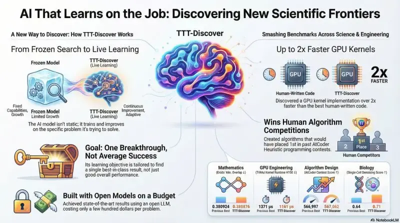
The current narrative in AI is dominated by “Inference Scaling”—the idea popularized by OpenAI’s o1 and DeepSeek’s R1. The premise is simple: give the model more time to “think” (generate hidden Chain of Thought tokens), and it gets smarter.

But there’s a fundamental limitation: The model’s brain is frozen.

No matter how long o1 thinks, its synaptic weights—the actual knowledge encoding—do not change. It is merely navigating a fixed map.

TTT-Discover (Test-Time Training to Discover), a new framework from Stanford and NVIDIA, breaks through this limitation. It proposes a radical shift: What if we let the model run gradient descent on the test problem itself?

This isn’t just “thinking”; this is real-time evolution. It’s the difference between a student trying to recall a formula during an exam versus a student who is allowed to open a textbook and learn a new chapter right in the middle of the test.

In this analysis, we will dissect how TTT-Discover works, why its “Mad Scientist” objective function is a game-changer, and how you can conceptually implement this logic.

The Core Philosophy: The “Mad Scientist” vs. The “Average Joe”

To understand TTT-Discover, you have to understand the difference between Chatbot RL and Discovery RL.

Standard RL (RLHF/PPO)

In standard training (like ChatGPT), the goal is to maximize the expected reward (average performance). You want the model to be generally helpful and rarely hallucinate.

Goal: Be consistently “okay” to “good.”
Math: $\max \mathbb{E}[R]$

TTT-Discover (Discovery RL)

In scientific discovery—whether finding a new sorting algorithm or a cure for a disease—we don’t care about the average. If a model tries 9,999 times and fails, but succeeds once on the 10,000th try, that is a total victory.

Goal: Find the single outlier; the “Black Swan.”
Math: $\max (\max R)$

TTT-Discover optimizes for the rare peak, not the safe average.

The Entropy Objective Function

The researchers introduced a specific objective function to achieve this. Instead of maximizing the average reward, they maximize the log of the expected exponentiated reward.

$$ J_\beta(\theta) = \mathbb{E}[\log \mathbb{E}[e^{\beta R}]] $$

Here is why this matters:

$\beta$ (Beta): This is a temperature-like parameter.
As $\beta \to \infty$: The objective function mathematically converges to maximizing the maximum possible reward.

It forces the model to ignore “safe” paths that yield mediocre rewards and instead aggressively update its weights toward paths that might yield a massive breakthrough, even if they are risky.

How It Works: The Loop

Unlike a standard inference call where you send a prompt and get a response, TTT-Discover is an iterative loop involving weight updates.

Sample: The model generates multiple potential solutions (trajectories) for the specific problem at hand.
Filter: It identifies high-potential steps using a modified search algorithm (PUCT).
Update: It calculates the gradient based on the “Mad Scientist” objective and updates the model’s weights temporarily.
Repeat: The model, now slightly smarter about this specific problem, tries again.

Conceptual Implementation

While the official codebase is complex, we can visualize the logic with a simplified PyTorch-style pseudo-code. This demonstrates how “Test-Time Training” differs from standard inference.

import torch
import torch.nn as nn
import torch.optim as optim

class TTTDiscoverAgent:
    def __init__(self, model, learning_rate=1e-5, beta=10.0):
        self.original_weights = model.state_dict() # Save the "frozen" brain
        self.model = model
        self.optimizer = optim.Adam(self.model.parameters(), lr=learning_rate)
        self.beta = beta

    def reset_model(self):
        """Reset to the original pre-trained state after solving a problem."""
        self.model.load_state_dict(self.original_weights)

    def discovery_loss(self, rewards):
        """
        The 'Mad Scientist' Loss.
        We want to maximize log(E[exp(beta * R)]).
        Since optimizers minimize loss, we take the negative.
        """
        # rewards: tensor of shape [batch_size]
        # We use LogSumExp trick for numerical stability
        scaled_rewards = self.beta * rewards
        log_expected_exp_reward = torch.logsumexp(scaled_rewards, dim=0) - torch.log(torch.tensor(len(rewards)))
        
        return -log_expected_exp_reward

    def solve(self, problem_input, iterations=100):
        """
        The Test-Time Training Loop
        """
        best_solution = None
        max_reward_seen = -float('inf')

        for i in range(iterations):
            self.optimizer.zero_grad()
            
            # 1. Generate multiple attempts (exploration)
            # In reality, this involves beam search or sampling
            outputs, log_probs = self.model.generate_with_grads(problem_input, num_samples=8)
            
            # 2. Evaluate attempts (External Verifier / Reward Model)
            rewards = self.evaluate_solutions(outputs)
            
            # Track best solution found so far
            current_max = torch.max(rewards)
            if current_max > max_reward_seen:
                max_reward_seen = current_max
                best_solution = outputs[torch.argmax(rewards)]
            
            # 3. Calculate Loss based on the Entropy Objective
            # Note: We need gradients flow through log_probs to update weights
            # This part is simplified; in PPO/TTT we use importance sampling or reparameterization
            loss = self.discovery_loss(rewards)
            
            # 4. UPDATE WEIGHTS (The Magic Step)
            loss.backward()
            self.optimizer.step()
            
            print(f"Iteration {i}: Max Reward = {max_reward_seen:.4f}")

        # Reset weights so the model doesn't overfit to this specific problem forever
        self.reset_model()
        return best_solution

    def evaluate_solutions(self, outputs):
        # Placeholder for a verifier (e.g., unit tests for code, formal verifier for math)
        return torch.randn(len(outputs))

Key Takeaway from Code: Notice the self.optimizer.step() inside the solve method. In standard RAG or Chain-of-Thought, this never happens. In TTT, the model is mutating to fit the problem.

The Secret Weapon: PUCT-Inspired State Reuse

Updating weights is risky. If the model finds a bad path and learns from it, it might collapse into generating garbage. To prevent this, TTT-Discover borrows from AlphaZero.

It uses a mechanism called PUCT (Predictor + Upper Confidence Bound applied to Trees).

Instead of just generating text linearly, the system maintains a “buffer” of promising states (partial solutions).

Component	Function
Q(s)	The quality of a state. Crucially, TTT uses the maximum reward of any child node, not the average.
P(s)	The prior probability (how likely the model thinks this step is good).
U(s)	The exploration term. It encourages visiting states that haven’t been visited much.

The Formula: $$ \text{Score}(s) = Q(s) + c \cdot P(s) \cdot \frac{\sqrt{\sum N}}{1 + N(s)} $$

In effect, the model can register that approach A failed, that approach B looked promising partway through, and then return to the middle of approach B, update its weights to favor that direction, and try again.

Real-World Applications: Why Should You Care?

This isn’t just academic gymnastics. The paper highlights applications that have direct industrial value.

1. GPU Kernel Optimization (The Billion Dollar Problem)

Writing CUDA kernels (the code that runs on NVIDIA GPUs) is notoriously difficult. It requires managing memory hierarchy, thread synchronization, and tensor cores.

The Task: Write a matrix multiplication kernel (like TriMul for AlphaFold or MLA for DeepSeek).
The Result: TTT-Discover, using an open-source model (gpt-oss-120b), generated kernels that outperformed those written by human experts.
Impact: A 5% speedup in a kernel used by a massive model translates to millions of dollars in saved electricity and compute time.

2. Open Mathematical Problems

The system was tested on the Erdős primitive set conjecture and other boundary value problems.

It didn’t just “solve” textbook problems; it improved the known bounds of these inequalities.
This proves the method can generate novel scientific knowledge, not just retrieve training data.

Critical Analysis: The Cost of Discovery

While TTT-Discover is impressive, we must look at the trade-offs.

The “Compute per Token” Explosion

We are moving from an era of “Training Compute” to “Inference Compute.”

Standard Inference: Cost is proportional to output length ($O(N)$).
CoT (o1): Cost is proportional to “thinking” length ($O(k \cdot N)$).
TTT-Discover: Cost is proportional to (Iterations $\times$ Backpropagation).

Backpropagation is significantly more expensive than forward inference (roughly 2-3x memory and compute). The paper mentions the cost per problem can reach hundreds of dollars. This is not for your “Write me an email” prompt. This is for “Design a new drug molecule” or “Optimize this high-frequency trading algorithm.”

The “Amnesia” Feature

Notice in the code above, we call reset_model(). TTT is usually episodic. The model learns intensely for Problem A, then forgets it all to tackle Problem B.

Pros: Prevents “catastrophic forgetting” of general knowledge.
Cons: The model doesn’t permanently get smarter. It’s a temporary boost.

Comparison: TTT vs. OpenAI o1

Feature	OpenAI o1 (Inference Scaling)	TTT-Discover (Test-Time Training)
Mechanism	Hidden Chain of Thought (CoT)	Gradient Updates on Test Instance
Weights	Frozen	Dynamic / Updated
Objective	Next-token prediction (mostly)	Maximize Peak Reward (Entropy)
Best For	Logic, Coding, General Reasoning	Scientific Discovery, Optimization
Cost	High	Very High

Conclusion: The Era of the Adaptive Model

TTT-Discover marks a shift in how we view Large Language Models. We are stopping treating them as static encyclopedias and starting to treat them as adaptive engines.

For developers and engineers, the takeaway is clear: The distinction between “training” and “inference” is blurring.

If you are building agents for high-value tasks (security auditing, chip design, financial modeling), simply prompting a frozen model—even a smart one like GPT-4—might soon be considered the “lazy” approach. The future belongs to agents that can practice, fail, learn, and evolve in the seconds before they give you an answer.

References: